
I have owned an electric bass for the last twenty five years. I managed to play it in the low 10s of hours and at some point could riff noises resembling the Pink Panther theme song. I decided it was time to get a band name matching my talent. Given that I am an engineer, I obviously automated the whole process.
This post explains how I trained a deep neural network to create new band names on demand. We will go over the training dataset generation process, we will review the model architecture, we will build intuition around what that model learned and we will use this model to generate new band names.
Band names dataset
I leveraged Wikidata and downloaded a dataset of music band names using the following sparql query:
SELECT DISTINCT ?entity ?bandName
WHERE
{
  ?entity wdt:P31/wdt:P279* wd:Q2088357.
  ?entity rdfs:label ?bandName.
  FILTER (LANG(?bandName) = 'en')
}
Here is a sample of what we get:
| entity | bandName |
|---|---|
| http://www.wikidata.org/entity/Q396 | U2 |
| http://www.wikidata.org/entity/Q371 | !!! |
| http://www.wikidata.org/entity/Q689 | Bastille |
| http://www.wikidata.org/entity/Q50598 | Infinite |
| http://www.wikidata.org/entity/Q18788 | Epik High |
For more details on how this works, please go through my previous post on dataset generation.
The resulting dataset contains 85,153 band names and 547 unique characters. Half of these characters are used only once or twice. Given that our model will have a hard time learning how to use rare characters and that each additional character makes the model slower to train, I took the following design decisions:
- All characters are lowercased;
- Only ASCII characters are included.
Using these two rules, I reduced the initial 547 characters to these 67:
{' ': 1,  '!': 2,  '"': 3,  '#': 4,  '$': 5,  '%': 6,  '&': 7,  "'": 8,
 '(': 9,  ')': 10, '*': 11, '+': 12, ',': 13, '-': 14, '.': 15, '/': 16,
 '0': 17, '1': 18, '2': 19, '3': 20, '4': 21, '5': 22, '6': 23, '7': 24,
 '8': 25, '9': 26, ':': 27, ';': 28, '=': 29, '?': 30, '@': 31, '[': 32,
'\\': 33, ']': 34, '^': 35, '_': 36, '`': 37, 'a': 38, 'b': 39, 'c': 40,
 'd': 41, 'e': 42, 'f': 43, 'g': 44, 'h': 45, 'i': 46, 'j': 47, 'k': 48,
 'l': 49, 'm': 50, 'n': 51, 'o': 52, 'p': 53, 'q': 54, 'r': 55, 's': 56,
 't': 57, 'u': 58, 'v': 59, 'w': 60, 'x': 61, 'y': 62, 'z': 63, '{': 64,
 '|': 65, '}': 66, '~': 67}
Using this alphabet, we can encode our band names to list of numbers that our model can understand:
In [22]: alphabet.encode("Glass Animals".lower())
Out[22]: [44, 49, 38, 56, 56, 1, 38, 51, 46, 50, 38, 49, 56]

In [23]: alphabet.encode("Arcade Fire".lower())
Out[23]: [38, 55, 40, 38, 41, 42, 1, 43, 46, 55, 42]
The number of band name we can represent from our dataset however drops from 85,153 to 79,753. Here are some of the names that can’t be spelled with this restricted alphabet:
Some of the characters in ASCII like ], ^ and \ are still used
only once in the dataset. We will live with this inefficiency for now.
Model architecture
Now that we have a dataset, we can teach a model to create new band names. I started from TensorFlow’s tutorial on text generation and poked around until I was satisfied. The result is this architecture:
model = tf.keras.Sequential(
    [
	# map each characters to an embedding of size 64
	tf.keras.layers.Embedding(
	    len(alphabet),
	    64,
	    batch_size=64,
	    mask_zero=True,
	),

	# we use 1,024 hidden units in our GRU.
	tf.keras.layers.GRU(
	    1024,
	    return_sequences=True,
	    stateful=True,
	    recurrent_initializer="glorot_uniform",
	),

	# predict a distribution over the next possible characters
	# knowing a prefix
	tf.keras.layers.Dense(len(alphabet)),
    ]
)
This model learns to write band names one character at a time. It is made of three building blocks which we will cover in more details:
-
A character embedding layer that maps characters into an embedding space;
-
A layer of Gated Recursive Units (GRUs) acting as a state machine writing band names one character at a time;
-
A densely connected layer estimating the probability of the next character from the state of the GRUs.
I trained this model using the sparse_categorical_crossentropy loss for eight epochs using mini-batch of size 64. Let’s look at what was learned in the process.
Character embeddings layer
The first layer of our neural network maps each character to an
embedding of size 64. Here is the embedding that was learned for the
character a (with index 38 according to our alphabet):
In [60]: model.layers[0].get_weights()[0][38]
Out[60]:
array([ 0.30702987, -0.63329417, -0.20212476, -0.4470627 ,  0.36042994,
       -0.49842888,  0.2777874 , -0.09102639,  0.19714546, -0.17154549,
       -0.21538487,  0.40895164,  0.37431315, -0.28506562, -0.44888547,
	0.7362037 , -0.15533094, -0.17730029,  0.36867294, -0.3623726 ,
       -0.24717565,  0.44966665,  0.2590245 , -0.3569541 ,  0.6784191 ,
	0.08784037, -0.43929407,  0.07683449,  0.00999499,  0.2224479 ,
       -0.32996455,  0.25540373,  0.436953  , -0.4415921 , -0.2441453 ,
       -0.21282889, -0.13839865, -0.5111227 ,  0.55712277,  0.11951732,
	0.05748424, -0.24553397,  0.5800741 ,  0.21185097, -0.2751697 ,
       -0.16367064, -0.5004835 , -0.3733032 ,  0.30201647, -0.25884396,
       -0.47911265, -0.26210967,  0.20878884, -0.35981387, -0.11836641,
	0.27695036, -0.10165487, -0.04859921, -0.4266084 ,  0.04561161,
	0.19834217, -0.59851754,  0.11871306, -0.3452472 ], dtype=float32)
Characters that are used similarly in band names should be close of
each other. For example, the 1 is probably closer to 2 than to
m. Let’s see if this intuition is supported by our data:
In [63]: embedding_1 = model.layers[0].get_weights()[0][18]
In [64]: embedding_2 = model.layers[0].get_weights()[0][19]
In [65]: embedding_m = model.layers[0].get_weights()[0][50]

In [68]: np.linalg.norm(embedding_1 - embedding_2)
Out[68]: 0.88233894

In [69]: np.linalg.norm(embedding_1 - embedding_m)
Out[69]: 3.327488

In [70]: np.linalg.norm(embedding_2 - embedding_m)
Out[70]: 3.3125098
We see that our embeddings are behaving as we expect. They put 1 and
2 close together while keeping m further away.
A more scalable way to visualize these distance is to use a tool like Embedding Projector. Here is what it looks like:
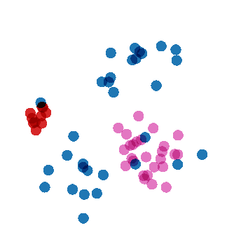
The red dots are all digits, the purple dots are letters and the blue
dots are other characters. We see that letters and digits are grouped
together as expected. There is also a blue dot for # hanging out
with the digits. Inspecting the band names with # we see that it is
used in the same context as number validating our intuition:
You can explore these embeddings yourself on Embedding Projector.
GRU layer
The GRU layer predicts the probability of a character being added to a prefix. We can express this probability as
\begin{equation} p(x_i | x_{i-1}, x_{i-2}, …, x_1) \end{equation}
and the probability of generating a band name as
\begin{equation} p(x_1^n) = \prod_{i = 1}^n p(x_i | x_{i-1}, x_{i-2}, …, x_1) \end{equation}
where \(x_1^n\) is a sequence of \(n\) characters and \(x_i\) is the i-th character in the sequence.
In traditional Natural Language Processing, we approximate the probability of adding a new character using the markovian assumption (we limit the state of the model to the last \(k\) characters):
\begin{equation} p(x_i | x_1^{i-1}) \approxeq p(x_i | x_{i-k}, x_{i - k + 1}, …, x_{i - 1}) \end{equation}
Since these models are trained using frequency tables, using small values of \(k\) helps fight data sparsity.
When using Gated Recurrent Units (GRU), we can condition our probability on the GRU’s state instead:
\begin{gather} gru_i = f(gru_{i-1}, x_{i-1}) \\ p(x_i | x_1, x_2, …, x_{i-1}) = p(x_i | gru_{i}) \end{gather}
where \(gru_{i-1}\) is a high dimension continuous state (i.e. an embedding) and \(f(\cdot, \cdot)\) is a state transition function learned by the model.
I mapped the final state of a sample our band name dataset using Embedding Projector:
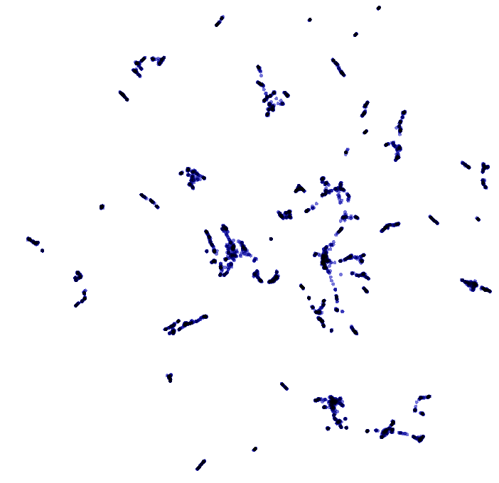
We observe many clusters of band names. If the markovian assumption is
helpful, band names ending with the same characters should be grouped
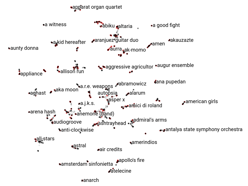
together. Here are all the bands ending with the letter a:
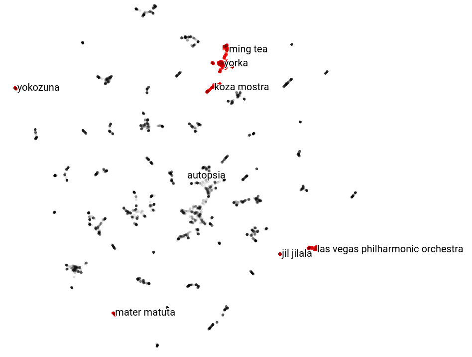
We observe that they are all grouped together in few clusters. Here is
the list of bands whose name ends with Cr's where we observe the same
thing:
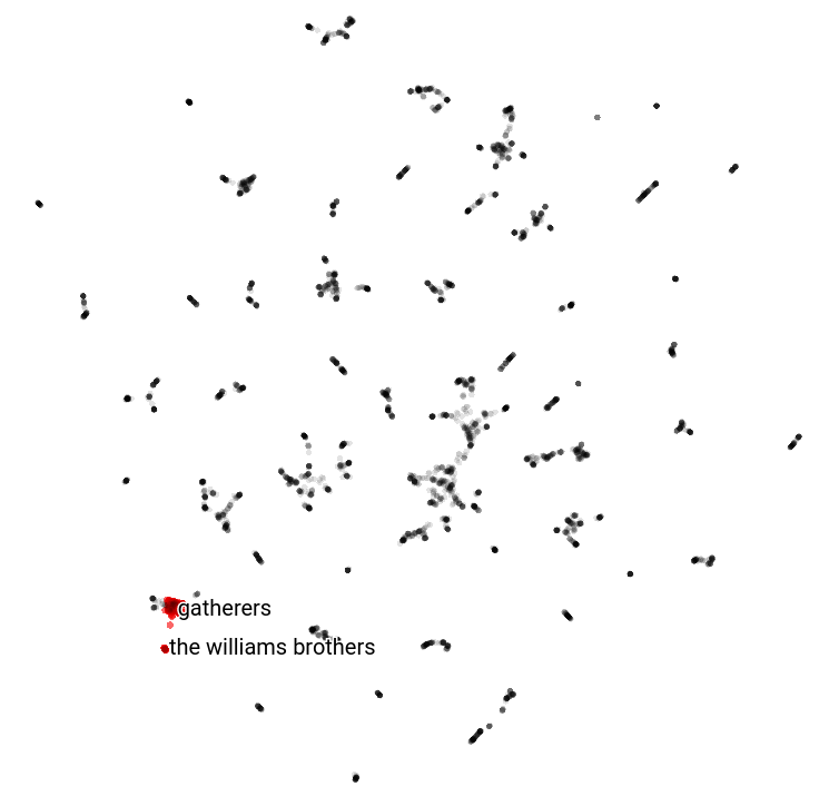
If we look at embeddings of bands with the same starting letter, we observe that it is all over the place:
We can also look at how a given band name embedding evolve as we are predicting letters. In this example, all red dots are states visited while generating the name glass animals:
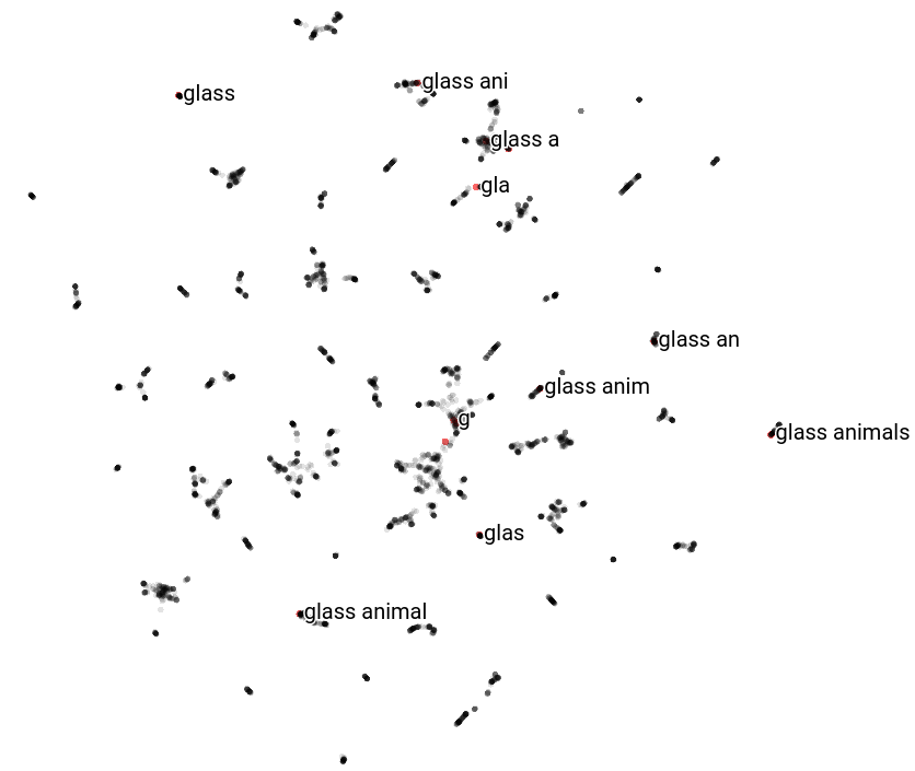
The state of the band name moves around, which supports our intuition that the GRU layer capture just enough of last few characters to help predict the next character.
Dense layer
The dense layer uses the GRU layer’s state to predict the likelihood of each character following the characters generated so far.
Creating new band names using the model
The model we trained gives us the probability of a character given a prefix. We use it in a decoding algorithm to generate band names one character at a time. The simplest decoding algorithms starts with a prefix and greedily sample characters one at a time:
def generate(
    model, prefix: List[int], eos: int, max_length: int):
    """
    Generate a sequence from a recurrent model.

    :param model: Model to generate the sequence with.
    :param prefix: Prefix to continue generating with the model.
    :param eos: Id to identify the end of a sequence (should be 0 most
	of the time).
    :param max_length: Maximum lenght of the sequence to generate.
    """
    output_values = []

    # Reset the state of the GRU layer (the embedding of the previous
    # prefix).
    model.reset_states()

    # Start with the provided prefix.
    input_values = tf.expand_dims(prefix, 0)
    output_values.extend(prefix)
    for i in range(max_length):
	# Compute the distribution over the next character. The
	# prediction will also affect the state of our GRU layers and
	# memorize the prefix embedding.
	predictions = model.predict(input_values, batch_size=1)
	predictions = tf.squeeze(predictions, 0)

	# Sample a character from this distribution.
	x_i = tf.random.categorical(predictions, num_samples=1)[-1, 0].numpy()

	if x_i == eos:
	    # This is the end of the name, we can return it.
	    break

	# Feed the prediction back into the model to predict the next
	# character.
	input_values = tf.expand_dims([x_i], 0)
	output_values.append(x_i)

    return output_values
I wrote a variant of this algorithm using beam search to generate the search graphs presented in the following section.
Results
I am now ready to pick a name for my band. I just need to prime the model with prefixes. Here is what the model outputted for a band name that starts with /rage /:
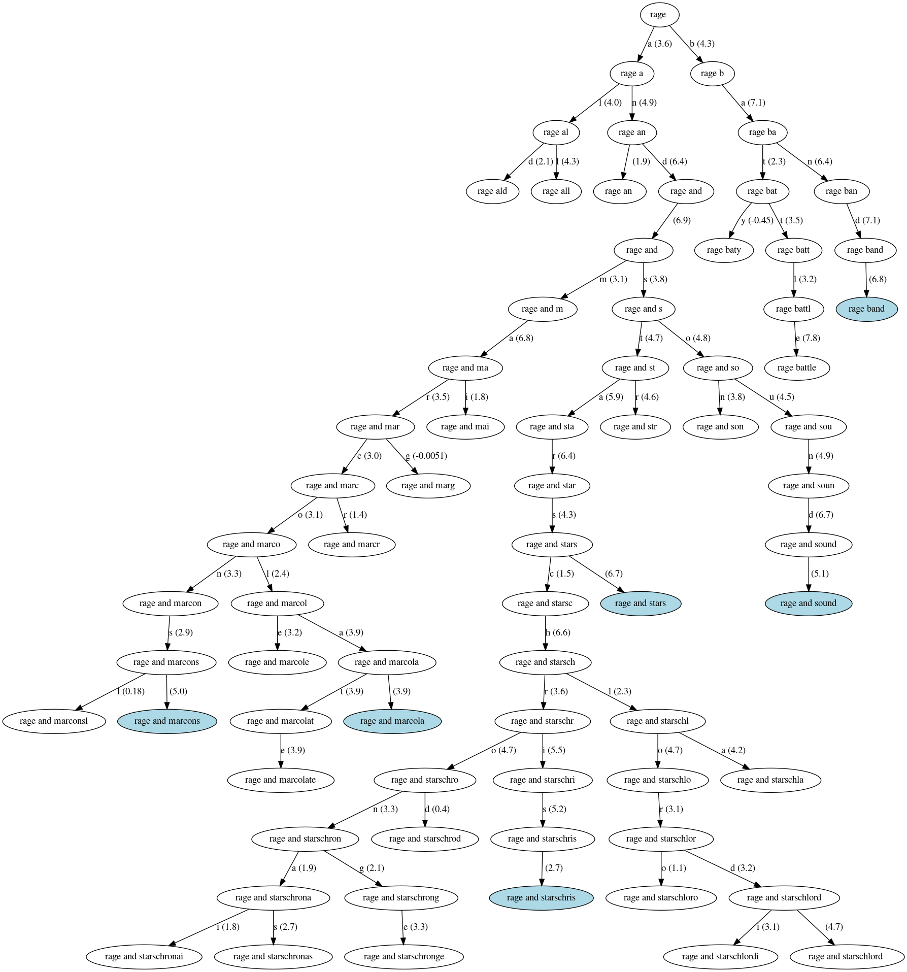
The white ellipses are partial band names that were dropped during the search and the blue ellipses are band names generated by the model. The edges are labeled with a character and its likelihood score.
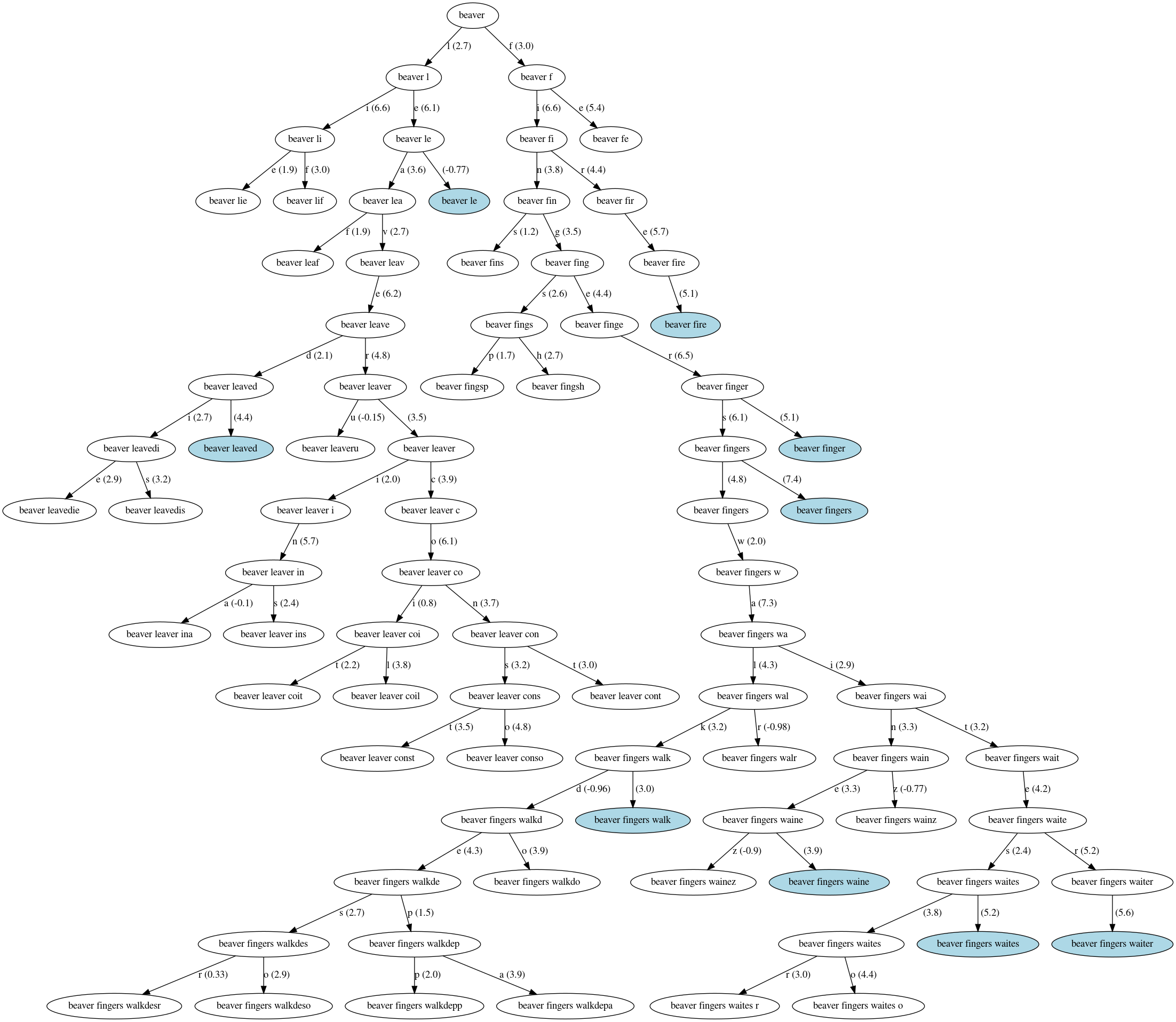
I am Canadian, I might as well have a band name starting with beaver:
Finally, I have options if I ever want a vanity project:
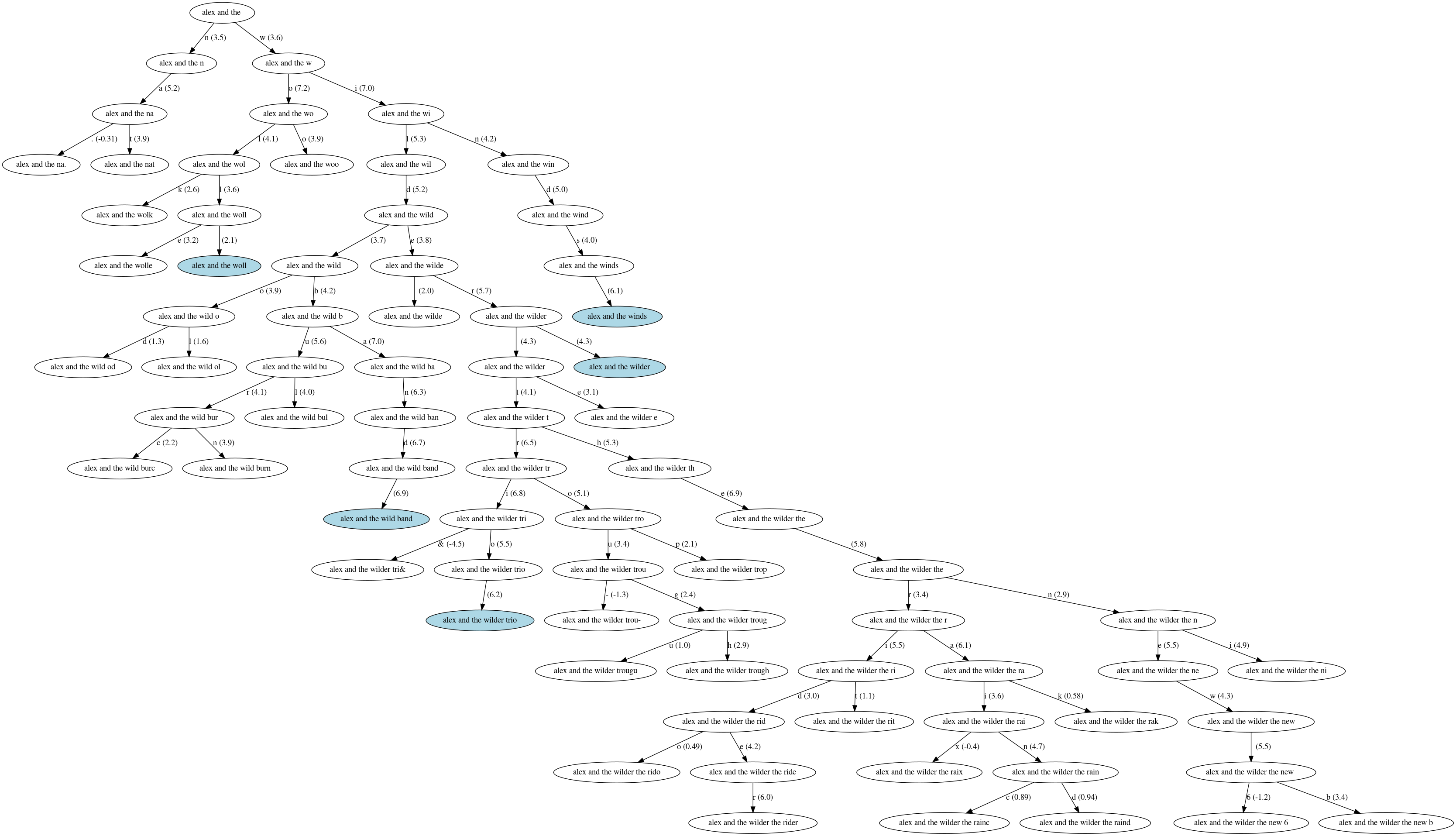
Given all of these options, my top three contenders are:
- Rage and Stars
- Beaver Fingers
- Alex and the Wilder Trio
I will go with a melancholic band names Rage and Stars but will keep Beaver Fingers in mind as a solid contender.
Wrapping up
We trained a model generating new band names from the following components:
-
A list of existing band names retrieved from Wikidata. I am extremely grateful to this project organizing advocating for an organized knowledge base in a world of embeddings.
-
A deep neural network generating text one character at a time. We saw that even if we use deep learning, we can still relate the model to classical Natural Language Processing approaches. The model learns to group characters into classes (e.g. digits and letters) and the model learns the markovian hypothesis by itself (i.e. state of words with the same suffix are grouped together). I am grateful for TensorFlow. It amazes me to see that what costed me sweat and blood to implement 12 years ago can now be done in few lines of Python.
-
A simple decoder that generate a band name one character at a time.
Organizing my code base for experimentation was more challenging than
I expected. I refactored two or three times and ended up with a mess
anyway. I am both happy and ashamed to share the it here. If
everything works as expected, you should be able to train your own
model using make bandaid PREFIXES="foo " on a fresh checkout.